Another statistical measure of variability, besides the interquartile range, can be used.
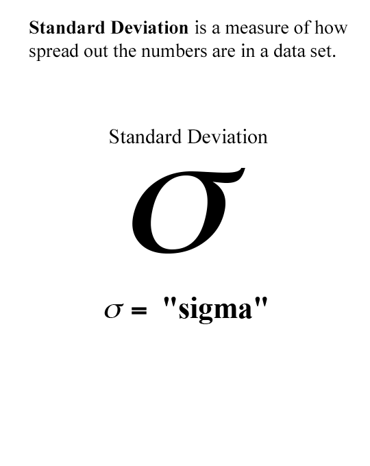
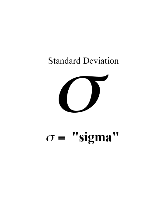
Standard Deviation is a measure of how spread out the numbers are in a data set. The symbol for standard deviation is the Greek letter sigma.
Standard deviation describes how much each value in a data set is above or below the mean, or how the data fall around the mean.
The greater the standard deviation of a data set, the more variable the data are. In other words, the data are further spread out away from the mean.
Smaller standard deviations mean less variable, more consistent data.
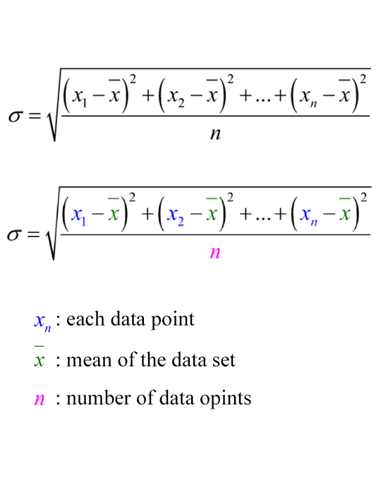
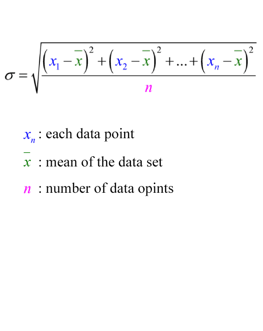
Standard deviation represents the average distance between individual data values and the mean (xx bar). It provides one number to represent the overall variability of the data.
The formula for calculating the standard deviation is shown.
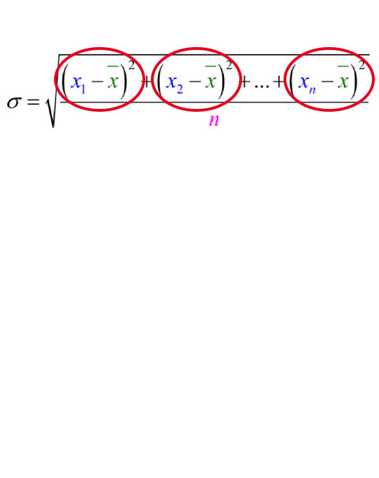
The difference between each data value and the mean (xn−x)the quantity of x sub n minus x bar is a measure of variability in the data.
Each value in the data set could be greater than the mean, (so the difference is a positive value), equal to the mean (so the difference is zero), or less than the mean (so the difference is a negative value).
If all these differences were added, they would sum to zero. Squaring allows us to keep the measures of variability.
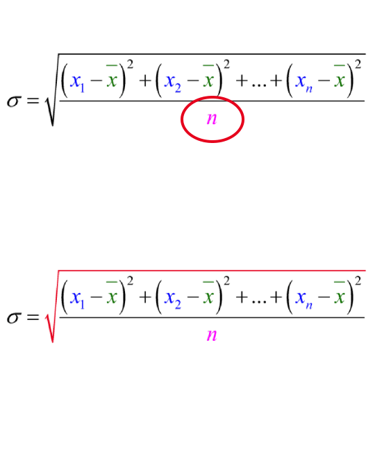
Dividing by n allows the standard deviation to be one number to represent the data set’s variability. It also allows us to use standard deviation to compare data sets of differing sizes.
Square rooting the entire quotient undoes the effects of squaring the differences.
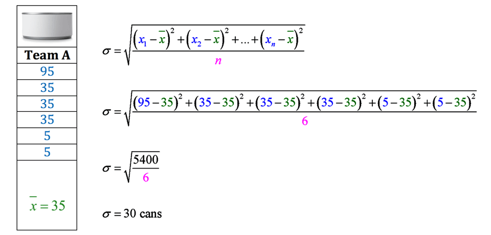
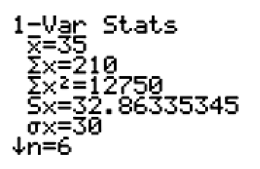
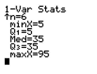
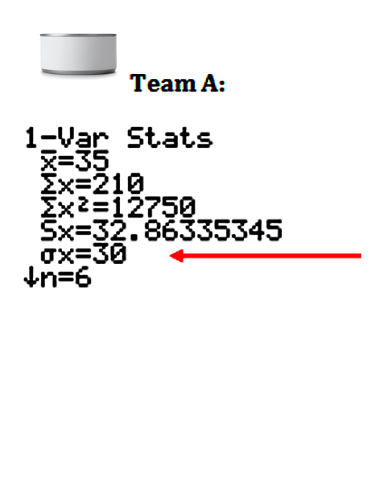
Here is the standard deviation for Team A from the food drive.
Team A has a standard deviation of 30 cans.
This means that, on average, a team member’s number of cans collected is about 30 cans from the mean amount of 35 cans.
The formula for standard deviation can be cumbersome and complicated.
Don’t worry!!
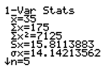
Under the one-variable statistics calculations in your graphing calculator, you will find that the standard deviation is calculated. There is no need to calculate it by hand.
Since the graphing calculator can easily calculate the standard deviation, it is more important to understand what the standard deviation tells us about the data.
Team A has a mean of 35 cans, with a standard deviation of 30 cans. A team member’s number of cans collected is, on average, about 30 cans from the mean amount of 35 cans.
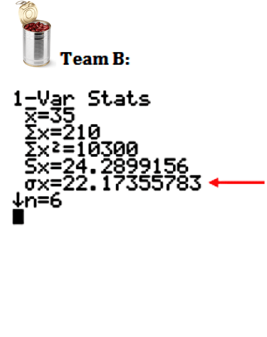
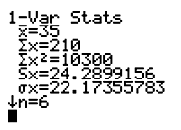
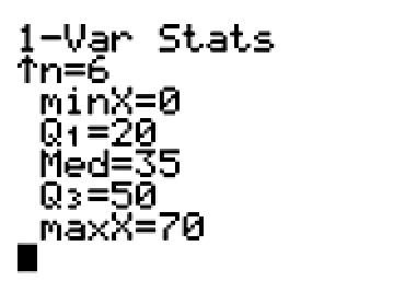
Team B has a mean of 35 cans, with a standard deviation of 22.17 cans. A team member’s number of cans collected is, on average, about 22 cans from the mean amount of 35 cans.
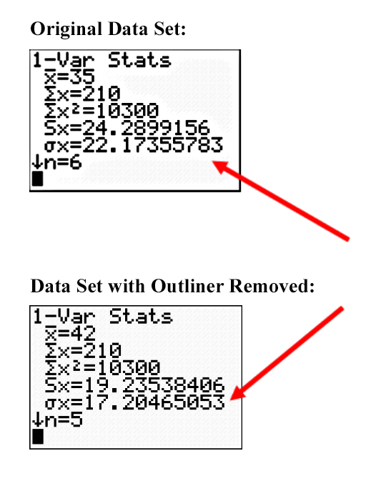
Standard deviation is sensitive to outliers, just like the mean. Standard deviation will be made larger if the data contains extreme values. This is because the data is more variable (more spread out).
Observe the changes in the value of the mean and standard deviation if the ‘0’ from Team B’s data set is removed. The data set is now less variable (closer together). This is shown by the smaller standard deviation.
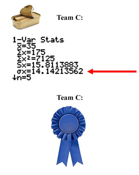
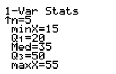
Team C has a mean of 35 cans, with a standard deviation of 14.14 cans. A team member’s number of cans collected is, on average, about 14 cans from the mean amount of 35 cans.
Since Team C has the lowest standard deviation, or the least variable data, we finally can conclude that the members of Team C worked together better than the other two teams
Team C should get the prize!

Still not convinced Team C should get the prize? Let’s take a look at the box and whisker plots for each team.
Notice how Team A is skewed right. This means that most of the data are on the left of the plot, but it stretches to the right because of the outliers. Team A had the largest standard deviation. When data are skewed and have outliers, the standard deviation tends to be large.
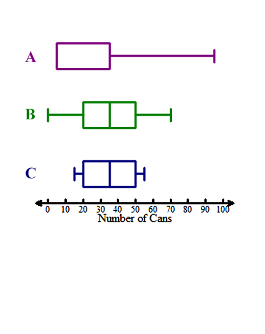
Team B is much less skewed than Team A, but notice how the left whisker is a bit longer than the right.
Team C has an even (normally) distributed box and whisker plot. The whiskers are the same size, and the box is the same size. Its data are not skewed, which means the data set is least variable. It has the smallest standard deviation, also.

The same distribution is shown in the histograms.
Data plots that fall equally to either side of the mean, in both quantity and value, are considered to be symmetrical.
Team A’s mean was 35 cans. Notice how a large group of the data falls below the 35 mark.
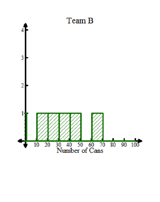
Team B’s mean was also 35 cans. Team B seems to have an equal amount of data to the left and right of the mean, but there is a large gap that happens between 50 and 60. It is not symmetrical.

Team C also had a mean of 35 cans. Notice how an equal number of bars are to the left and the right of the 35 mark? The bars show an equal amount of data to the left and right, with no gaps. Note that in a histogram, the bars don’t have to be equal in size, but corresponding bars should be approximately the same height. This happens with Team C. Team C is the most consistent team, and deserves the prize.
 Team A
 Team B