Correctly analyzing data helps us make informative projections and estimates.
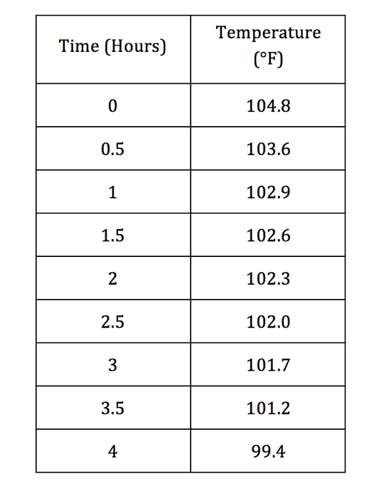
The data in the table shows a patient’s temperature over time after taking medication to reduce fever.
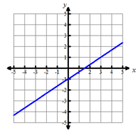
What function family does the data appear to model?
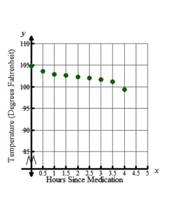
This data appears to follow a linear association between the hours since the medication was given and the temperature of the patient.
How can we find the linear equation that best fits this data?
Curve fitting is a process of determining the equation of a function that best fits the data given. A regression analysis will determine how well the curve fits the data by averaging how far each data point is from the estimated curve.
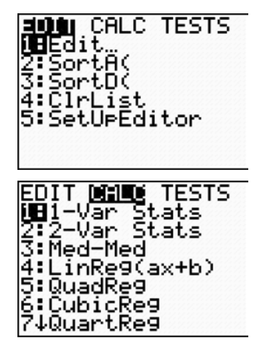
The graphing calculator can perform the curve fitting and the regression analysis of the data by helping us determine which type of function—linear, quadratic or exponential—is the best fit for modeling the data.
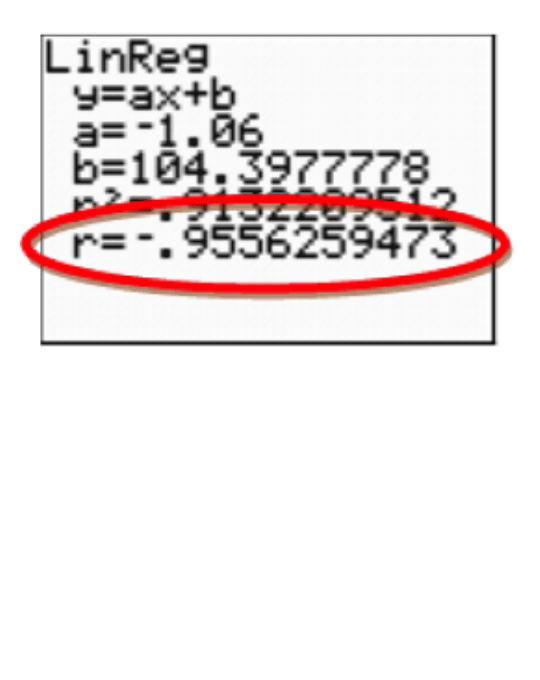
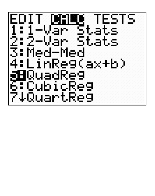
Option 4, LinReg(ax+b), will perform a linear regression.
Option 5, QuadReg, will perform a quadratic regression.
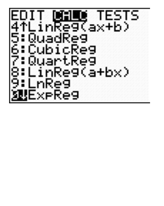
Option 0, ExpReg, will perform an exponential regression.
(To activate these windows on the TI-84 calculator, press STAT and then press the right arrow to activate the CALC menu.)
Since the data appears to be linear, let’s do a linear regression.
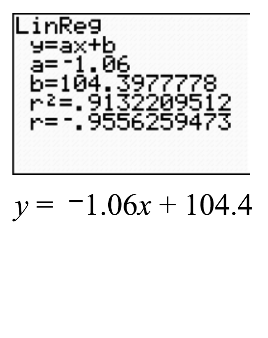
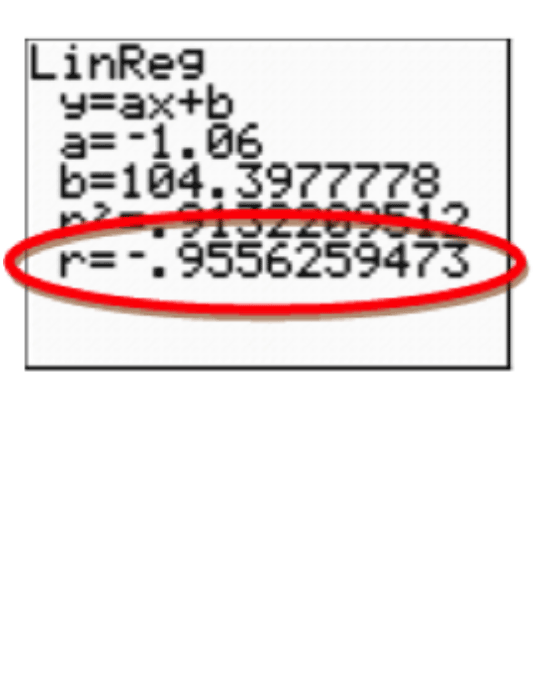
Performing a linear regression on the temperature data shows these results.
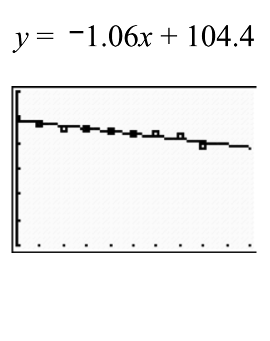
The linear equation
y = -negative1.06x + 104.4
y equals negative one and six hundredths x plus one hundred four and four tenths. fits the data.
We can use this regression equation to make the following conclusions:
The slope of the equation is -negative1.06. This means the patient’s temperature is dropping approximately 1.06 degrees each hour since the medication was administered.
The y intercept is 104.4°F. This means the patient’s temperature was about 104.4°F before the medication was administered.

By substituting the value of 98.6°F in for y, we can find out approximately when the patient’s temperature will return to normal.

 After about 5.47 hours, the patient’s temperature should return to normal.
How reliable is this equation? How well does this linear equation fit the data?
A correlation coefficient is a measurement of how well a regression line fits the data. It averages how far each data point is from the regression line.
The correlation coefficient is the r value given by the calculator when a regression calculation is performed.
The value of the correlation coefficient is always between -negative1 and 1. The closer the value is to -negative1 or 1, the better the fit. The closer the value is to 0, the worse the fit.
If the correlation coefficient is negative, then the correlation between the variables in the data is also negative. This means that as the independent variable increases, the dependent variable decreases (that is, as the x values increase, the y values decrease).
If the correlation coefficient is positive, then the correlation between the variables in the data is also positive. This means that as the independent variable increases, the dependent variable increases (that is, as the x values increase, the y values increase).
For the temperature data, the correlation coefficient is -negative0.9556. This value is extremely close to -negative1, and confirms a very strong linear association between the temperature of the patient and the hours after medication. Since the correlation between these two variables is negative, we can conclude that as the time increases, the temperature decreases.
A linear equation is a strong fit for the data.
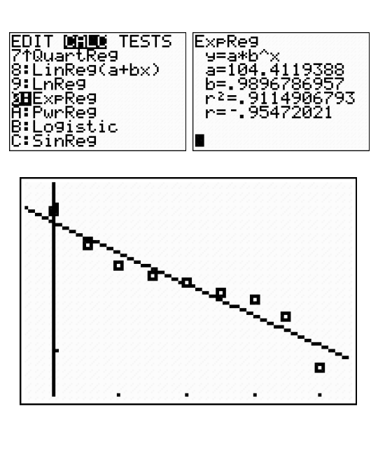
If we had chosen an exponential regression, the correlation coefficient is not as strong. It is only -negative0.9547.
This means an exponential curve would be a poor fit for the data.
We will talk more about quadratic regressions a little later in this module. (A quadratic regression includes an additional calculation called the coefficient of determination, which we will need to discuss in detail.)
Our linear equation was a strong fit! The conclusions we made about the slope and y-intercept are statistically sound conclusions. The data value we extrapolated is reliable.